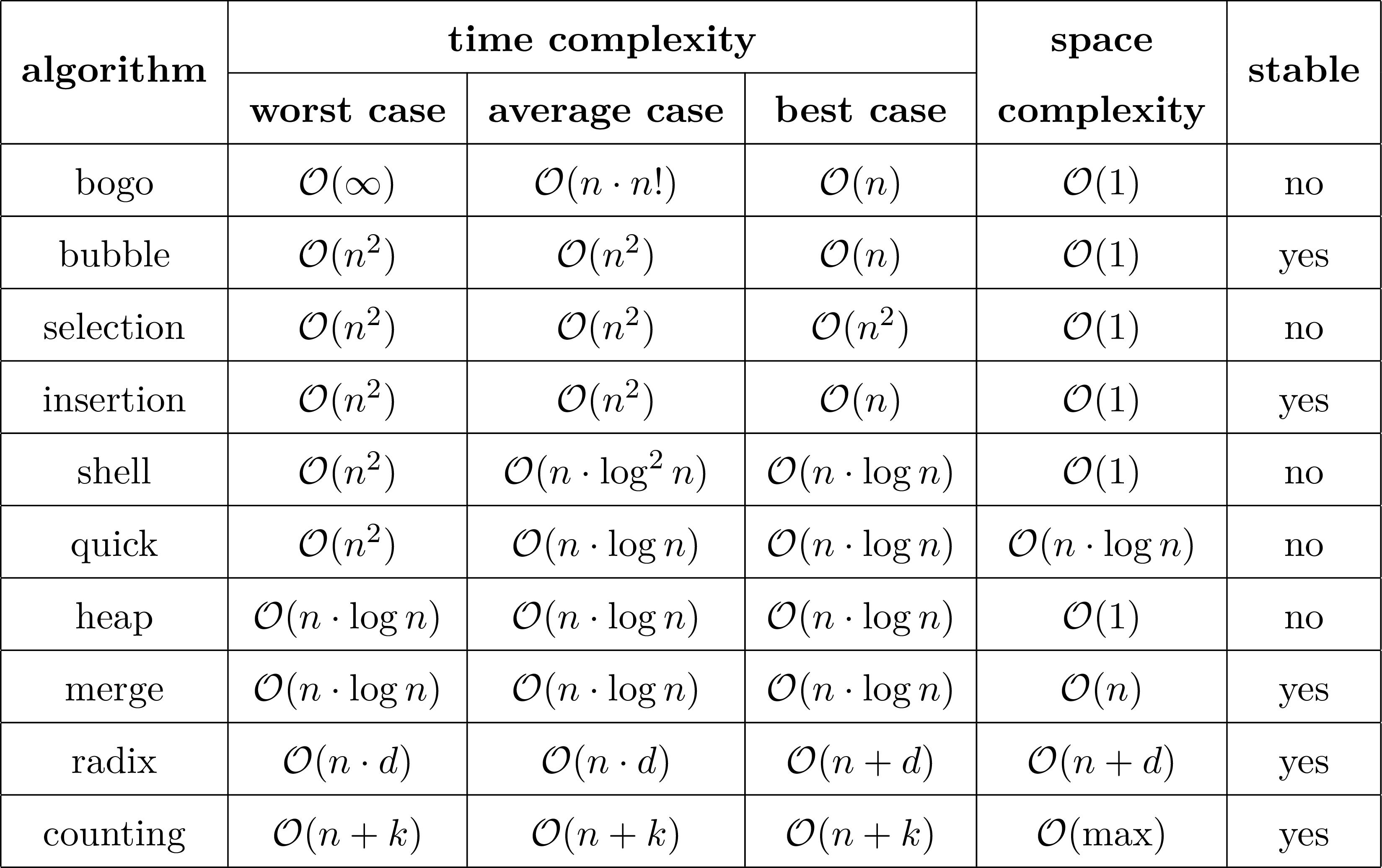
\(n:\) number of elements
\(d:\) number of digits of the largest element
\(k:\) difference between largest and smallest element
max\(:\) largest element
\(\require{mathtools}\)
By \(\mathcal{O}(f(n))\), spoken "big O of f(n)", we denote the upper bound of time
and space
complexity of our sorting algorithms.
Mathematically, let \(f:\mathbb{N}\rightarrow\mathbb{N}\) be a (computable)
function, then we define \[\mathcal{O}(f(n))\coloneqq\{g(n) \;|\; \exists c,N>0:
g(n)\leq c\cdot f(n) \forall n\geq N\}.\]
Intuitively we say \(g(n)\in\mathcal{O}(f(n))\) or \(g(n)=\mathcal{O}(f(n))\)
whenever
\(f\) grows asymptotically at least as fast as \(g\).
For example, \(\mathcal{O}(1)\subseteq\mathcal{O}(\log
n)\subseteq\mathcal{O}(n)\subseteq\cdots\)
A sorting algorithm is called stable if the initial order of equal elements
is
preserved. When sorting the array \([4,3_a,1,3_b,2]\), a stable sorting algorithm
would output \([1,2,3_a,3_b,4]\), whereas an unstable one might output
\([1,2,3_b,3_a,4]\).